Capital Efficiency Explained: Optimize Your Portfolio in Stock & Index Trading

​​

Introduction to Capital Efficiency

Capital efficiency is how efficiently each dollar invested generates a return. When thinking about capital efficiency, it's not just the total profits, but what type of returns you are getting from the capital you are investing. It's similar to "miles per gallon" when considering an investment, referring to your return per dollar invested. 

Why is capital efficiency even worth considering? When capital efficiency improves, it reduces the amount of capital you have tied up to achieve similar or better returns. This frees up money for other opportunities, lowers your single position risk exposure, and allows you more flexibility in your trading decisions.  

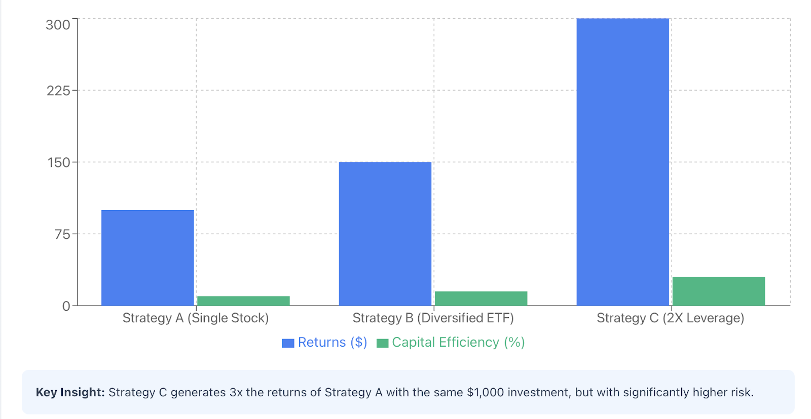
Let's go through three strategies with a $1,000 investment:

Strategy A: Buy and hold a single stock that grows at 10% annually. This strategy generates $100 in return with capped capital efficiency of 10%.  

Strategy B: Diversified portfolio of ETF's with rebalancing every quarter and generating 15% in returns will produce a 15% capital efficiency ($150 returns).   

Strategy C:  A combination of well-placed 2X leverage, risk parameters, and prudent methodology yields returns that push the 15% return to 30% capital efficiency, but increases the risk.  

As you can imagine, professional portfolio fund managers are obsessed with capital efficiency considering things like portfolio allocation, complicated hedge strategies, and leverage with the right amount of risk parameters. Having a capital efficiency mindset as an individual trader can improve your trading ability and methods significantly in a stock, ETF, and/or index fund position. 

Calculating Capital Efficiency: Essential Metrics

You cannot manage what you do not measure. There are several factors or metrics, whether qualitative or quantitative, that illuminate the actual level of performance of your strategy, beyond simple percentage gain in 12 months (or any other duration).

The Basic Theory

Capital Efficiency = Total Returns + Invested Capital

For example, if you invested $5,000 and generated a return of $750, your capital efficiency is 15%. However, this primitive calculation does not take risk into account.

The Sharpe Ratio: Risk v Returns

The Sharpe ratio indicates return v risk levels:

Sharpe Ratio = Portfolio Return - Risk free rate ÷ Standard deviation of returns

An example would be:

• The portfolio generated a return of 12%

• The risk free (e.g., treasury bill) is 3%,

• The standard deviation of the portfolio is 10%

• Sharpe Ratio = (12% - 3%) ÷ 10% = .9

Generally, any Sharpe ratio over 1.0 is considered good, over 2.0 is excellent, and over 3.0 is considered very good. Values above 3.0 indicate return per unit of risk.

Return on Capital Employed (ROCE) calculation follows: 

ROCE = Net Returns divided by (Initial Capital plus Margin Used).  

In the last example, using $10,000 of initial capital, a margin used of $5,000, and net returns of $2,250 provides a ROCE of $2,250 ÷ $15,000 = 15%. This information reveals a full picture of efficiency when leverage is incorporated. 

Maximum Drawdown: The Pain Metric

Maximum drawdown provides the greatest peak-to-trough decline. If your portfolio reached a peak of $12,000 before bottoming out at $9,000, your maximum drawdown would be 25%. When comparing two portfolio draws with similar returns, capital efficiency would favor the portfolio with a lower drawdown.

The Nasdaq strategy offers the potential for higher returns, but that greater return comes with increased volatility and larger drawdowns. The Sharpe Ratio is a common metric for determining whether a strategy providing more returns is worth the additional risk taken.

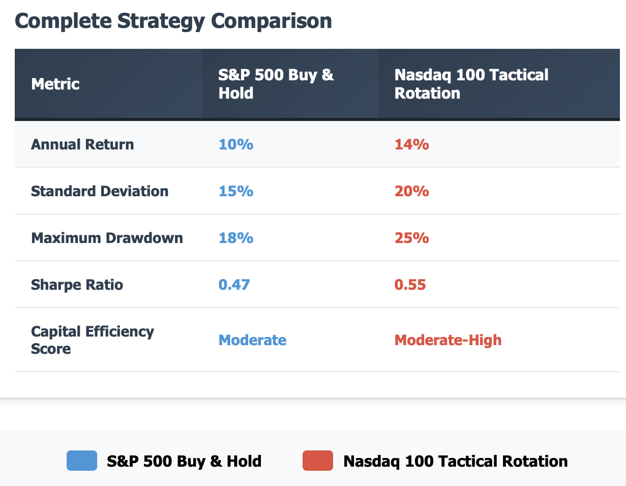
Key Takeaway: A strategy that provides you 20% returns and 40% volatility with a 35% peak drawdown is not nearly as capital efficient as a strategy that provides you 15% returns and 12% volatility with a 10% peak drawdown. You must always think of your returns relative to the risk taken.

Optimisation Strategies: What works

1. Leverage and Margin

Leverage allows you to significantly enhance your capital efficiency because you can control a much larger position that would normally require significantly more cash to do so. However, leverage can destroy accounts quickly if you do not use it properly.

Beginner Example:

Supposing you have $5,000 in capital:

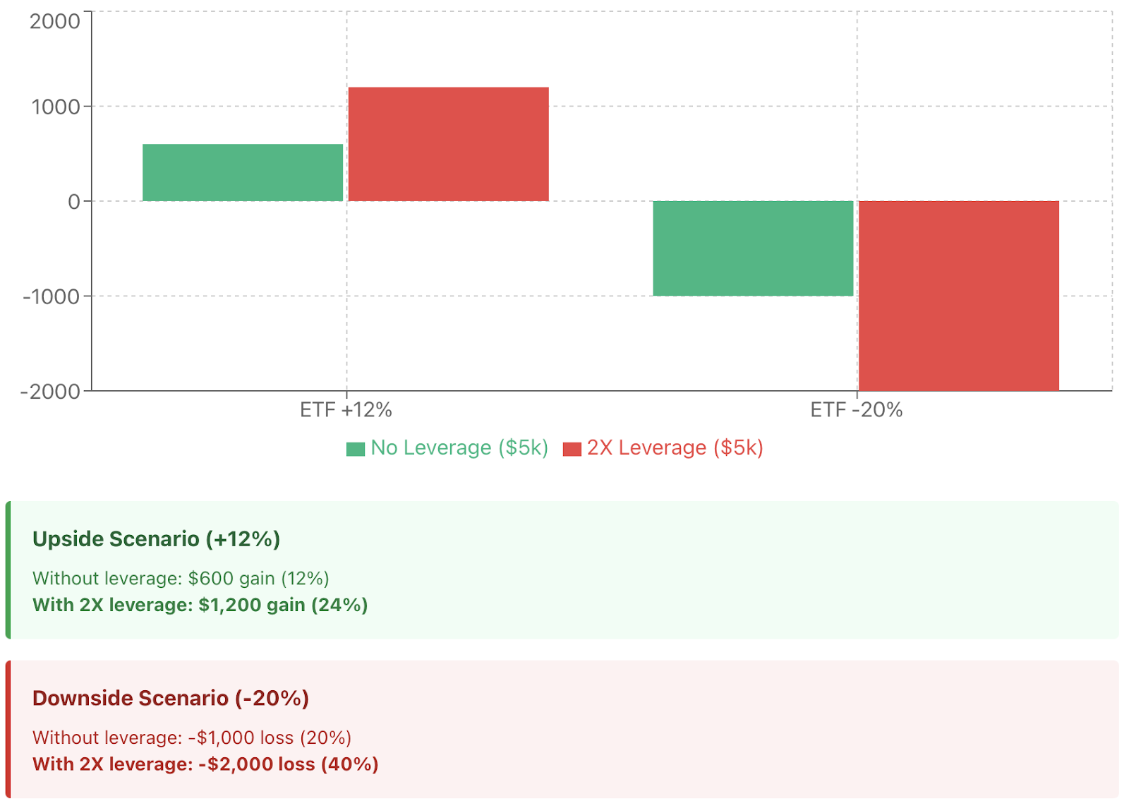
• No Leverage: Invest the $5,000 into an S&P 500 ETF which grows 12% annually. Your position will turn to $5,600. Capital efficiency is 12%

• Leverage 2x: In that same ETF, you use your $5,000 to control a 10,000 dollar position. The same ETF growing at 12% turns to 12k or $1,200 gains on your initial $5,000 in capital. Capital efficiency in this trade is 12% (1200/5000 = .24)

• The downside is if the ETF dropped by 20% your $5,000 puts you down minus $1,000 with 20% (20% loss) or down $2,000 of your total capital with the 2x leverage (40% loss) moviing your account to $3,000.

Risk Control Considerations:

• Stop losses should be strictly set before the trade and should be the maximum total capital loss of 2-3% per position.

• Start your trades with 1.5 leverage and progress from there

• Use a ratio suitable for the volatility of the asset being traded

• Calmly monitor your trade if you are in leverage.

2. Portfolio Allocation Optimisation

Diversifying can decrease volatility and help preserve growth; this, ultimately increases risk-adjusted returns.

Beginner Example: Three ETF portfolio

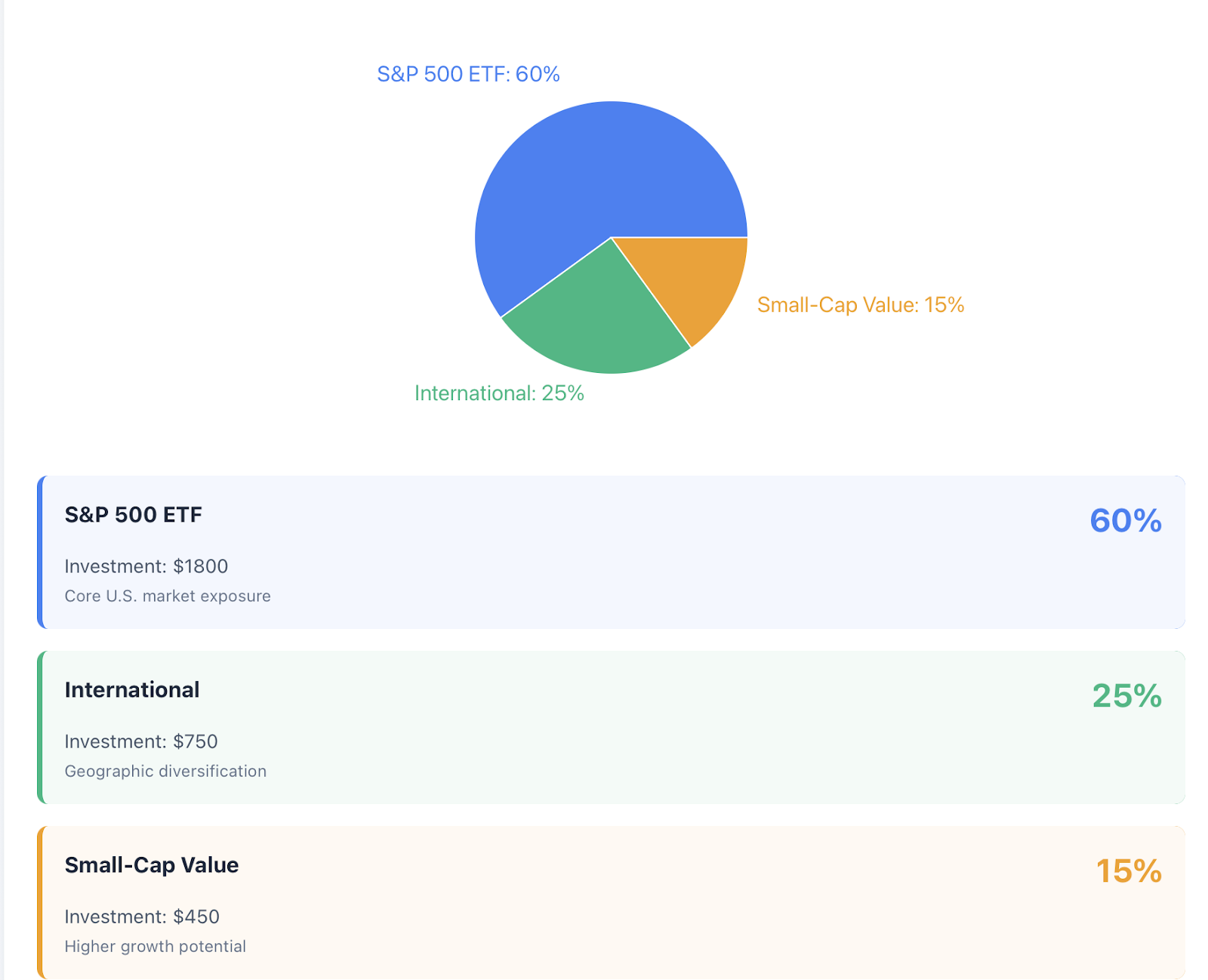
The starting point with $3,000:

• 60% ($1,800): S&P 500 ETF (VOO/SPY), this is your core U.S. exposure

• 25% ($750): Internationally developed markets (VEA/IEFA), this is your geographic diversification

• 15% ($450): Small-cap value (VBR/IJS), this is your higher growth potential

 

This allocation typically provides 80-90% of market returns with 15-20% less volatility. Over simulated 5-year periods, this is a potential return of 11% per annum, with 13% volatility (Sharpe Ratio: 0.85), compared to 12% return with 16% volatility (Sharpe Ratio: 0.75) for all-S&P 500 portfolios.

Advanced Strategies:

• Factor tilts: overweight value, momentum, or quality stocks

• Strategic satellite positions: add 10-15% to high-conviction sectors

• Correlation analysis: own assets that behave independently of each other

3. Regular Rebalancing

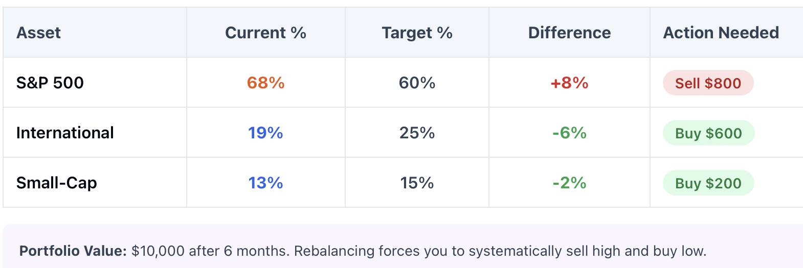
The market drifts; this means your 60/25/15 allocation now might develop to 68/20/12 as holdings perform differently. Rebalancing is forcing a systematic sell-high, buy low.

Rebalancing Frequency:

• Every quarter: for active traders who are watching closely

• Every six months: a healthy compromise

• Once a year: bare minimum, to stay hands-off

When your allocation is outside of your target by 5% or more

 

Example for the beginner:

• You have a $10,000 portfolio after 6 months.

• Your S&P 500 allocation is $6,800 (68% of overall portfolio) Target: 60%

• Your International allocation is $1,900 (19% of overall portfolio) Target: 25%

• Your Small-Cap allocation is $1,300 (13% of overall portfolio) Target: 15%

• You would rebalance by taking $800 off your S&P 500 and putting $600 into International and $200 into Small-Cap.

 

Having discipline to do this can potentially add 0.5-1.5% to your annualized returns, thus enhancing your overall capital efficiency.

4. Professional-Level Techniques

• ETF Arbitrage: The practice allows you to exploit the price discrepancies between the market price of an ETF and its net asset value. In order to arbitrage the differences requires significant cash along with real-time information regarding price movements.

• Options Hedging: By utilizing covered calls on your S&P 500 positions, you can obtain an additional 1-2% income per month, which increases your effective return on the same initial capital.

• Index Futures: You're allowed to control the equivalent of approximately $250,000 worth of stocks using E-mini-S&P 500 futures by utilizing a required margin of approximately $12,000-15,000. That's 17:1 leverage along with significant expert risk management requirements.

Risk Management and Stress Testing

Scenario Simulation

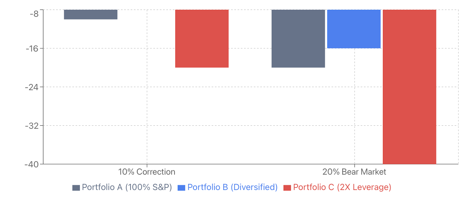
10% Correction:

• Portfolio A (100% S&P 500): $10,000 → $9,000 (10% loss)

• Portfolio B (diversified three-ETF): $10,000 → $9,200 (8% loss)

• Portfolio C (2x leveraged S&P 500): $10,000 → $8,000 (20% loss)

20% Bear Market:

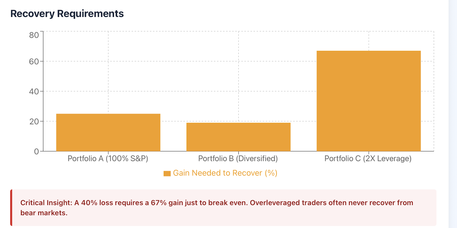
• Portfolio A: $10,000 → $8,000 (needs 25% gain to recover)

• Portfolio B: $10,000 → $8,400 (needs 19% gain to recover)

• Portfolio C: $10,000 → $6,000 (needs 67% gain to recover)

Overleveraged traders often never recover from bear markets.

Maximum Drawdown Guidelines

• Conservative Investors: Should seek to manage MDD below 15%.

• Moderate Investors: Should be willing to accept MDD between 15-25%.

• Aggressive Investors: Should be comfortable with an MDD between 25-35%.

• Above MDD of 35% = extreme risk and possibly requiring a re-evaluation of investment strategy.

Developing a Risk Process

• Step 1: No individual pose or allocation should be higher than 10% in total portfolio (an individual stock could be 5%).

• Step 2: Utilize stop-loss orders. A fixed stop-loss in a range (7-10%), likely a trailing stop (travelling 10% below the peak the stock reaches) or using technical stops (below support levels). 

• Step 3: Perform health check quarterly on portfolio allocations and when reviewing the performance of your positions monthly. This would include, allocation, performance, Sharpe Ratio, max drawdown, among other things.

• Step 4: Conduct 3 risk stress tests quarterly, accounting for 10% corrections, 20% bear market and a sector fall or interest rate increases.

Real-World Case Studies

Vanguard's Balanced Portfolio

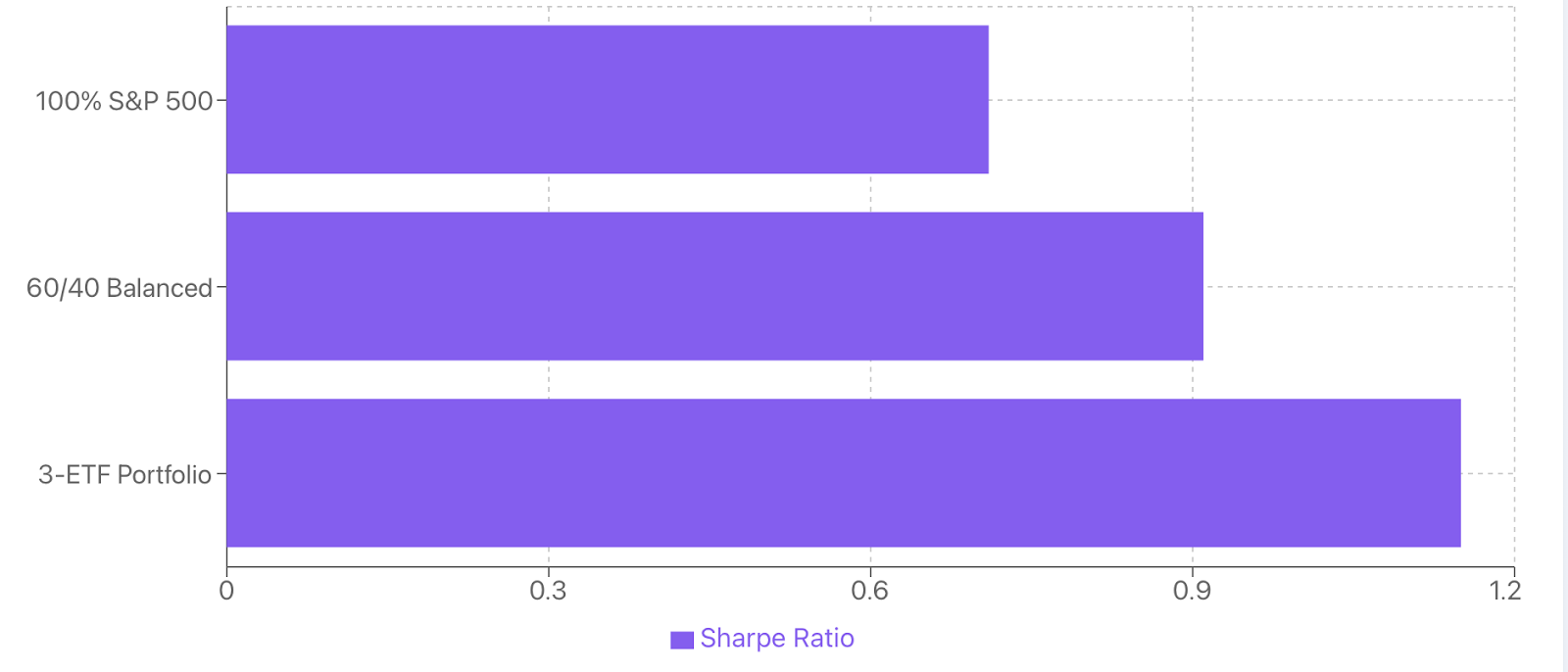
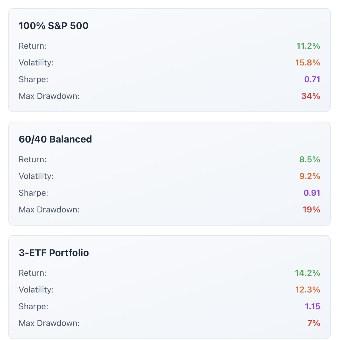
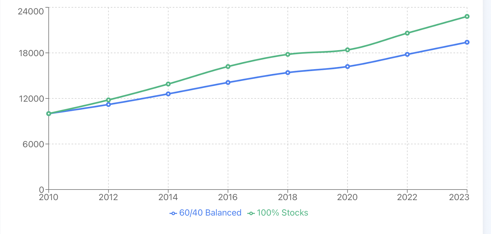
Vanguard's classic 60/40 portfolio (60% stocks, 40% bonds) demonstrates time-tested capital efficiency:

Historical Performance (2010-2023):

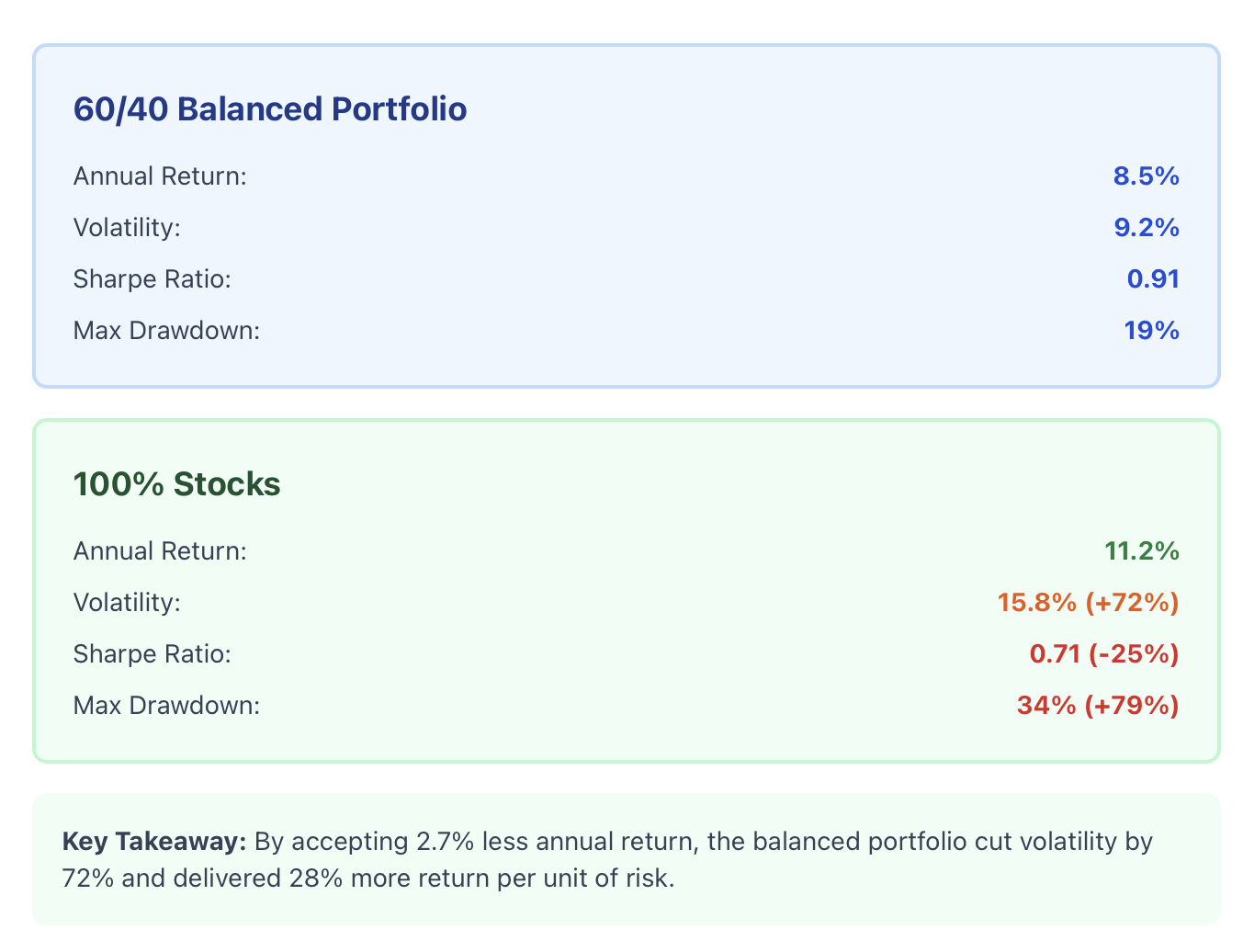
• Average annual return: 8.5%

• Standard deviation: 9.2%

• Sharpe Ratio: 0.91

• Maximum Drawdown: 19%

Compared to 100% stocks:

• Return: 11.2% (2.7% higher)

• Volatility: 15.8% (72% more)

• Sharpe Ratio: 0.71 (25% less efficient)

• Max Drawdown: 34% (79% larger)

By accepting 2.7% less annual return, the balanced portfolio cut volatility by 72% and maximum drawdown nearly in half, delivering 28% more return per unit of risk.

Beginner's $1,000 Portfolio

Year 1 Results:

• Starting: $1,000 in three-ETF portfolio

• Ending value: $1,142

• Total return: 14.2%

• Maximum drawdown: 7%

• Sharpe Ratio: 1.15

vs. S&P 500 only:

• Ending value: $1,135

• Return: 13.5%

• Max drawdown: 9%

• Sharpe Ratio: 0.95

The diversified approach delivered higher returns with 22% less drawdown and superior Sharpe Ratio - capital efficiency in action.

Actionable Implementation Steps

Begin with Simulation

Use Tradewill to practice without risking any live capital.

90 Day Action Plan:

Month 1: Set up simulation, build simulated portfolio, log daily, read basic literature.

Month 2: Experiment with rebalancing strategies, calculate initial Sharpe Ratio, run stress tests.

Month 3: Open brokerage - Transfer $500-$1000 to preferences from broker, transfer strategy to live account and execute some trades.

 

Build out the roll stock tracking system

Create Google sheets to log all typically: date, current value of portfolio, assets, returns, standard deviation, Sharpe ratio, and maximum drawdown. Log each week.

Avoiding typical pitfalls

• Overtrading: Too many trades destroy returns in Fees/taxes. 

• Chasing performance: Last year's winner is often this year loser.

• Ignoring costs & fees: Only invest in ETFs with maximum expense ratios of <0.20%

• Leverage too soon: Effective unleveraged performance strategy takes 3-5 years before introducing your first leverage position. 

• Follow your system: If you have an effective strategy - stick to it despite all the fear & greed emotions.

Conclusion

Capital efficiency changes investing from speculation to systematic wealth creation. You have learned how to measure efficiency with Sharpe Ratio and max drawdown, you have learned to implement time-tested tactics from diversification to meaningful rebalancing, oiling risk with stress testing, as well as taking lessons from real-life examples.

The market rewards discipline, consistency, and intelligent risk management and punishes impulsivity and inefficiency. A strategy earning 12% every year with low volatility significantly beats a strategy earning 30% one year, and losing 20% the next.

Start today. Open a simulation account, build your first three-fund portfolio, track results for one month, then gradually expand skills. Prioritise risk-adjusted returns over raw performance. Your future wealth depends on actions taken today; stop leaving returns on the table through inefficient capital deployment.